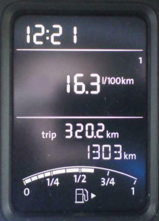
In the previous chapter we started from the relative velocity, this time we briefly take the momentary velocity. How can we best approach it? Of course by driving. But since the speedometer is deliberately designed to be relatively sluggish, we will instead look at the current consumption. So we change the center display and off we go.

By the way, this is a valuable exercise to handle the accelerator pedal a little more calmly, because you will now see constantly jumping values. Anything seems possible, from zero to over 20 litres/100km. On a long If we look at the distance, the instantaneous velocity is the same as the average velocity. Estimate your average after such a tour. Bets, you are a lot too high?

Can you imagine what a digital output of the instantaneous speed would look like, possibly with one digit behind the comma? We did that once with a homemade improvised tachometer. Terrible, hard to read. Corrections are made all the time. Where we finally landed? With the hundreds. So it was enough for us, only each change around hundred revolutions per minute.

And why do we mention the momentary speed here, when it is so difficult to capture? Because all speeds in the motor vehicle sector basically only exist as points, perhaps even when we think we're driving uniformly across the freeway. Also a cruise control has a lower and an upper limit, which must be reached first, so that it becomes active.

Here you can see the fluctuations of the piston speed during one revolution. The small fluctuations between about 90 and 270° result from the short connecting rods that are common today. Physics must therefore proceed point by point. So we assume a recording of the speed as above, a continuously changing line in height.

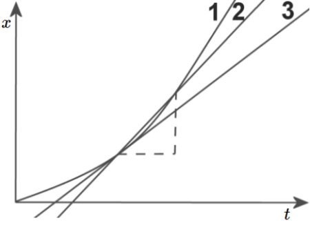
The diagram shows the line of the slowly increasing speed (curve 1). The point for which we want to determine the instantaneous velocity is marked by the left end of the horizontal dashed line. We start from the upper corner point on the vertical dashed line. The connection between the two points is secant 2, which becomes tangent 3 when the upper point on curve 1 is moved downwards.

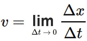
Their gradient would reflect the instantaneous velocity. The time difference must go towards zero, the two dashed lines must become smaller and smaller. This is shown by equation above which belongs to the differential calculus where such calculations are performed. Although we have determined the velocity in a point, there is still a vector of the instantaneous velocity with the direction represented by the tangent and the magnitude of the calculated velocity at this point.

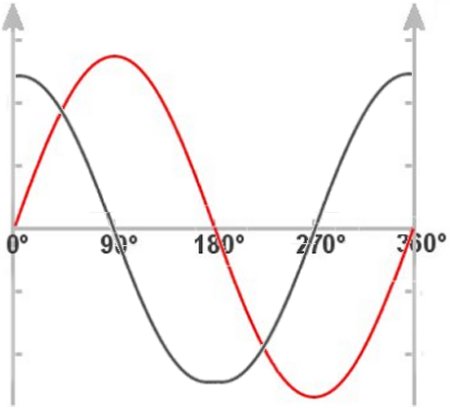
If this was still a very short connecting rod further up, we have an infinitely long one here to make it a little easier. The piston speed is more smoothed. It remains at the zero crossing at 0, 180 and 360°. The second curve represents the acceleration. This decreases from 0 to 90°, of course, but very rapidly at the end. If the piston reaches the dead center, the acceleration is zero. Then it rises again, but in the other direction.

The acceleration indicates the change in speed. Its unit is m/s², which means the increase of a certain speed in m/s in every second. This too is often assumed to be constant for greatly simplified calculations in automotive engineering. Do you really think a vehicle has the same deceleration, the reversal of acceleration, from 200 to 100 km/h as from 100 to 0 km/h?

The graphical calculation of the instantaneous acceleration is very similar to that of the instantaneous velocity and of course the acceleration can be displayed as a vector again. Our subject however is again like at previous chapter force. The way this time starting from the acceleration is again found in a Newtonian axiom, this time the second one.

Because according to Newton, the force is equal to the mass multipied by the acceleration. Mass has been added here, which can be explained relatively easily again with motor vehicle technology. Have you ever pushed a car before? Did you notice the difference between a heavy and a light car? Then you may also be able to estimate the difference when a light or a heavy car hits an obstacle without braking.

Exactly this connection is described in Newton's second axiom, of course neglecting any losses. Once pushed to a degree plane, the car runs and runs and runs. The force is reflected in the speed generated by acceleration, which in turn is inversely proportional to the mass of the vehicle.